


1 Mechanics
1.1 Forces, Moments and Couples
1.1.1 Scalar and Vector Quantities
Before introducing force as a measurable quantity, we should discuss how we identify that quantity.
Quantities are thought of as being either scalar or vector. The term scalar means that the quantity possesses magnitude (size) ONLY. Examples of scalar quantities include mass, time, temperature, length etc. These quantities, as the name “scalar” indicates, may only be represented graphically to some form of scale.
THUS
a temperature of 15°C may be
represented as:
Fig 2.1 Scalar representation of 15ºC
Vector quantities are different in that they possess both magnitude AND direction and, if either change, the vector quantity changes. Vector quantities include force, velocity and any quantity formed from these.
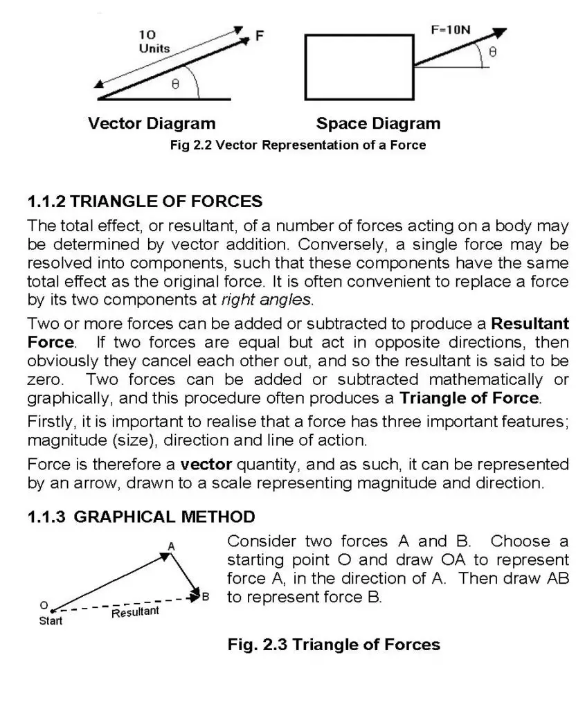
A force is a vector quantity, and as such, possesses magnitude and direction. In specifying a force, therefore, you must specify both the size of the force and the direction in which it is applied. This can be shown on a diagram by a line of a specific length with the direction indicated by an arrow. The most convenient method is to represent the force by means of a vector as shown in the diagram. If the point of application of a force is important it may be shown in a space diagram.
Vector Diagram Space Diagram
Fig 2.2 Vector Representation of a Force
1.1.2 Triangle of Forces
The total effect, or resultant, of a number of forces acting on a body may be determined by vector addition. Conversely, a single force may be resolved into components, such that these components have the same total effect as the original force. It is often convenient to replace a force by its two components at right angles.
Two or more forces can be added or subtracted to produce a Resultant Force. If two forces are equal but act in opposite directions, then obviously they cancel each other out, and so the resultant is said to be zero. Two forces can be added or subtracted mathematically or graphically, and this procedure often produces a Triangle of Force.
Firstly, it is important to realise that a force has three important features; magnitude (size), direction and line of action.
Force is therefore a vector quantity, and as such, it can be represented by an arrow, drawn to a scale representing magnitude and direction.
1.1.3 Graphical Method
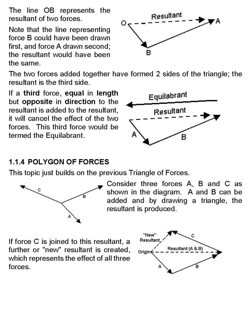
Consider two forces A and B. Choose a starting point O and draw OA to represent force A, in the direction of A. Then draw AB to represent force B.
Fig. 2.3 Triangle of Forces
The line OB represents the resultant of two forces.
Note that the line representing force B could have been drawn first, and force A drawn second; the resultant would have been the same.
The two forces added together have formed 2 sides of the triangle; the resultant is the third side.
If a third force, equal in length but opposite in direction to the resultant is added to the resultant, it will cancel the effect of the two forces. This third force would be termed the Equilabrant.
1.1.4 Polygon of Forces
This topic just builds on the previous Triangle of Forces.
Consider three forces A, B and C as shown in the diagram. A and B can be added and by drawing a triangle, the resultant is produced.
If force C is joined to this resultant, a further or “new” resultant is created, which represents the effect of all three forces.
Now this procedure can be repeated
many times; the effect is to
produce a Polygon of Forces[SJ1] .
1.1.5 Coplanar Forces
Forces whose lines of action all lie in the same plane are called coplanar forces. The following laws relating to coplanar forces are of importance and should be noted carefully. However, it must also be remembered that these laws are applicable ONLY to two dimensional problems.
The line of action of the resultant of any two coplanar forces must pass through the point of intersection of the lines of action of the two forces.
If any number of coplanar forces act on a body and are not in equilibrium, then they can always be reduced to a single resultant force and a couple.
If three forces acting on a body are in equilibrium, then their lines of action must be concurrent, – that is, they must all pass through the same point.
Forces acting at the same point are called CONCURRENT forces.
1.1.6 Effect of an Applied Force
If a Force is applied to a body, it will cause that body to move or rotate. A body that is already moving will change its speed or direction. Note that the term ‘change its speed or direction’ implies that an acceleration has taken place.
This is usually summarised in the formula; F = ma
Where F is the force, m = mass of body and a = acceleration.
The units of force should be kg.m/s2 but the SI Unit used is the Newton.
Hence, “A Newton is the unit of force that when applied to a mass of 1 kg. causes that mass to accelerate at a rate of 1 m/s2.
Applied forces can also cause changes in shape or size of a body, which is important when analysing the behaviour of materials.
1.1.7 Equilibriums
Earlier it was defined that a force applied to a body would cause that body to accelerate or change direction.
If at any stage a system of forces is applied to a body, such that their resultant is zero, then that body will not accelerate or change direction. The system of forces and the body are said to be in the equilibrium.
Note: This does not mean that there are no forces acting; it is just that their total resultant or effect is zero.
1.1.8 Resolution of Forces
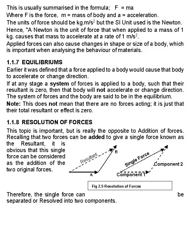
This topic is important, but is really the opposite to Addition of forces. Recalling that two forces can be added to give a single force known as the Resultant, it is obvious that this single force can be considered as the addition of the two original forces.
Therefore, the single force can be separated or Resolved into two components.
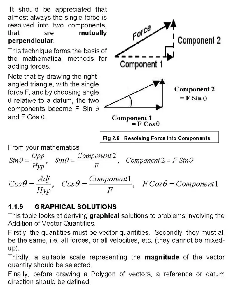
It should be appreciated that almost always the single force is resolved into two components, that are mutually perpendicular.
This technique forms the basis of the mathematical methods for adding forces.
Note that by drawing the right-angled triangle, with the single force F, and by choosing angle q relative to a datum, the two components become F Sin q and F Cos q.
From your mathematics,
1.1.9 Graphical Solutions
This topic looks at deriving graphical solutions to problems involving the Addition of Vector Quantities.
Firstly, the quantities must be vector quantities. Secondly, they must all be the same, i.e. all forces, or all velocities, etc. (they cannot be mixed-up).
Thirdly, a suitable scale representing the magnitude of the vector quantity should be selected.
Finally, before drawing a Polygon of vectors, a reference or datum direction should be defined.
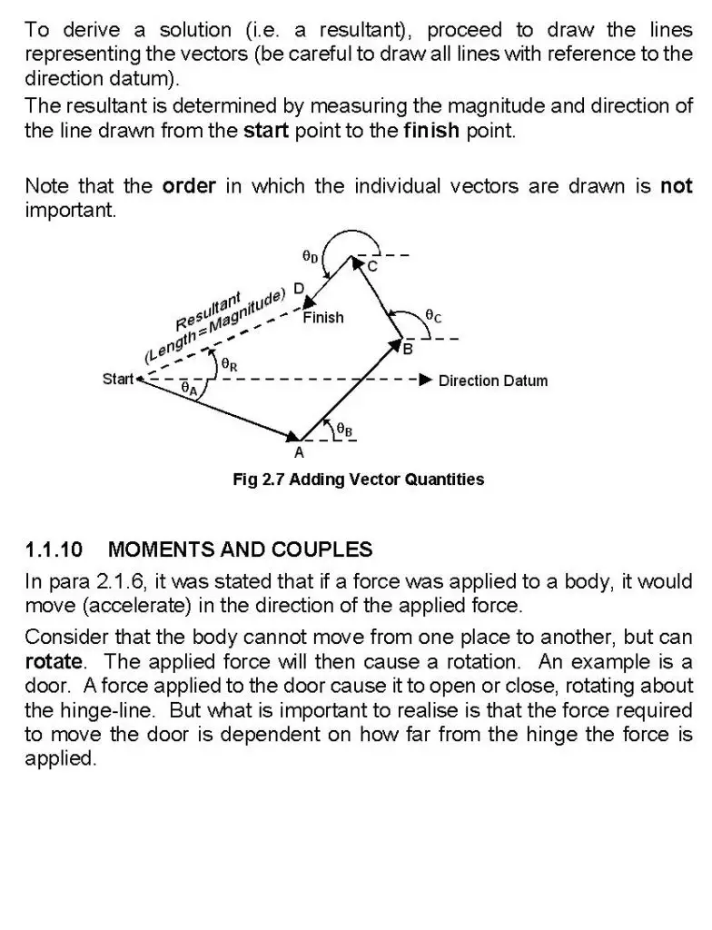
To derive a solution (i.e. a resultant), proceed to draw the lines representing the vectors (be careful to draw all lines with reference to the direction datum).
The resultant is determined by measuring the magnitude and direction of the line drawn from the start point to the finish point.
Note that the order in which the individual vectors are drawn is not important.
Fig 2.7 Adding Vector Quantities
1.1.10 Moments and Couples
In para 2.1.6, it was stated that if a force was applied to a body, it would move (accelerate) in the direction of the applied force.
Consider that the body cannot move from one place to another, but can rotate. The applied force will then cause a rotation. An example is a door. A force applied to the door cause it to open or close, rotating about the hinge-line. But what is important to realise is that the force required to move the door is dependent on how far from the hinge the force is applied.
So the turning effect of a force is a combination of the magnitude of the force and its distance from the point of rotation. The turning effect is termed the Moment of a Force.
From the diagram it can be seen that the moment is a result of the formula:
Moment of a force (F) about a point (O) = F x y
[where ‘y’ is the perpendicular distance between the force and the point ‘O’ often referred to as the ‘moment arm’ ].
Using SI units, the units are Newton x metres = Newton Metres or Nm
Note: It is important to realise that the “distance” is perpendicular to the line of action of the force.
1.1.11 Clockwise and Anti-Clockwise Moments
Fig 2.9 Clockwise and Anti-Clockwise Moments
The moment or turning effect of a force about a specific point can be clockwise or anti-clockwise depending on the direction of the force. In the diagram shown, Force B produces a clockwise moment about point O and Force A produces an anti-clockwise moment.
When several forces are involved, equilibrium concerns not just the forces, but moments as well. If equilibrium exists, then clockwise (positive) moments are balanced by anticlockwise (negative) moments. It is normal to say:
Clockwise Moments = Anti-clockwise Moments
Beam Example 1:
The diagram shows a light beam pivoted at point B with vertical forces of 50N and 125N acting at the ends. The 50N force produces an anti-clockwise moment of 50 x 3 = 150Nm about point B and the 125N force produces a clockwise moment of 125 x Y = 125Y Nm.
Fig 2.10 Simple Beam
If the beam is in equilibrium, Clockwise moments = Anti-clockwise moments, so:
125Y = 150, or Y = 1.2m
Note: In the previous beam example, if the beam is in equilibrium, we have stated that the CWM = ACWM. As well as this, the total force acting downwards, must equal the total upwards force. There is a vertical “reaction” acting at point B. The magnitude of this reaction is equal to the sum of the other two forces i.e. 175N. We do not need to include this value in the calculation, because it does not produce a turning moment if we assume the beam is pivoted at this point. (175 x 0m = 0Nm)
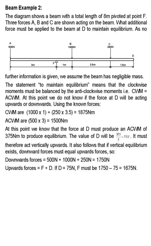
Beam Example 2:
The diagram shows a beam with a total
length of 8m pivoted at point F. Three forces A, B and C are shown acting on
the beam. What additional force must be applied to the beam at D to maintain
equilibrium. As no further information is given, we assume the beam has
negligible mass.
The statement “to maintain equilibrium” means that the clockwise moments must be balanced by the anti-clockwise moments i.e. CWM = ACWM. At this point we do not know if the force at D will be acting upwards or downwards. Using the known forces:
CWM are (1000 x 1) + (250 x 3.5) = 1875Nm
ACWM are (500 x 3) = 1500Nm
At this point we know that the force at D must produce an ACWM of 375Nm to produce equilibrium. The value of D will be . It must therefore act vertically upwards. It also follows that if vertical equilibrium exists, downward forces must equal upwards forces, so:
Downwards forces = 500N + 1000N + 250N = 1750N
Upwards forces = F + D. If D = 75N, F must be 1750 – 75 = 1675N.
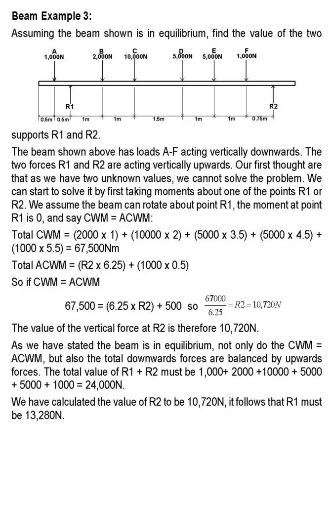
Beam Example 3:
Assuming the beam shown is in
equilibrium, find the value of the two supports R1 and R2.
The beam shown above has loads A-F acting vertically downwards. The two forces R1 and R2 are acting vertically upwards. Our first thought are that as we have two unknown values, we cannot solve the problem. We can start to solve it by first taking moments about one of the points R1 or R2. We assume the beam can rotate about point R1, the moment at point R1 is 0, and say CWM = ACWM:
Total CWM = (2000 x 1) + (10000 x 2) + (5000 x 3.5) + (5000 x 4.5) + (1000 x 5.5) = 67,500Nm
Total ACWM = (R2 x 6.25) + (1000 x 0.5)
So if CWM = ACWM
67,500 = (6.25 x R2) + 500 so
The value of the vertical force at R2 is therefore 10,720N.
As we have stated the beam is in equilibrium, not only do the CWM = ACWM, but also the total downwards forces are balanced by upwards forces. The total value of R1 + R2 must be 1,000+ 2000 +10000 + 5000 + 5000 + 1000 = 24,000N.
We have calculated the value of R2 to be 10,720N, it follows that R1 must be 13,280N.
1.1.12 Couples
When two equal but opposite forces are present, whose lines of action are not coincident, then they cause a rotation.
Together, they are termed a Couple, and the moment of a couple is equal to the magnitude of a force F, multiplied by the distance between them.
The basic principles of moments and couples are used extensively in aircraft engineering
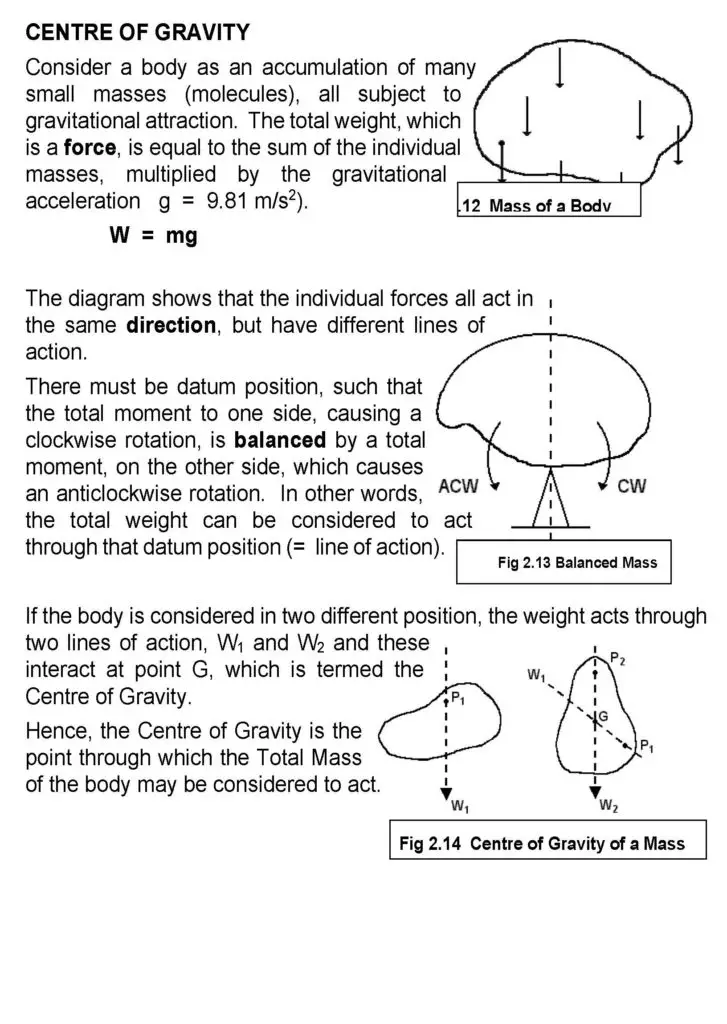
centre of gravity
Consider a body as an accumulation of many small masses (molecules), all subject to gravitational attraction. The total weight, which is a force, is equal to the sum of the individual masses, multiplied by the gravitational acceleration g = 9.81 m/s2).
W = mg
The diagram shows that the individual forces all act in the same direction, but have different lines of action.
There must be datum position, such that the total moment to one side, causing a clockwise rotation, is balanced by a total moment, on the other side, which causes an anticlockwise rotation. In other words, the total weight can be considered to act through that datum position (= line of action).
If the body is considered in two different position, the weight acts through two lines of action, W1 and W2 and these interact at point G, which is termed the Centre of Gravity.
Hence, the Centre of Gravity is the point through which the Total Mass of the body may be considered to act.
For a 3-dimensional body, the centre of gravity can be determined practically
by several methods, such as by measuring and equating moments, and this is done
when calculating Weight and Balance of aircraft.
A 2-dimensional body (one of negligible thickness) is termed a lamina, which only has area (not volume). The point G is then termed a Centroid. If a lamina is suspended from point P, the centroid G will hang vertically below ‘P1’. If suspended from P2 G will hang below P2. Position G is at the intersection as shown.
A regular lamina, such as a rectangle, has its centre of gravity at the intersection of the diagonals.
A triangle has its centre of gravity at the intersection of the medians.
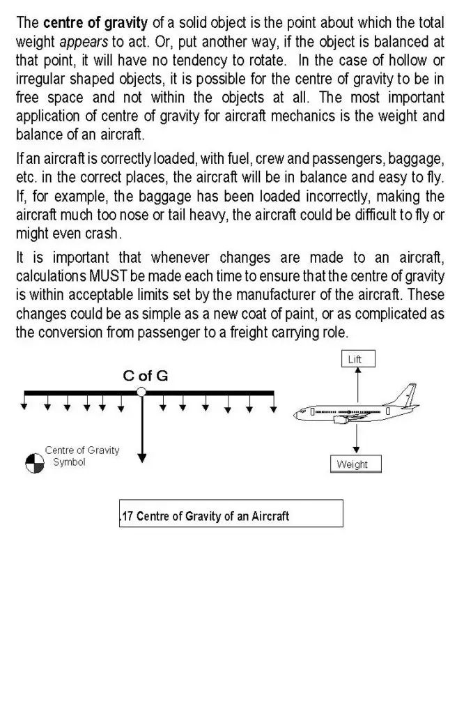
The centre of gravity of a solid object is the point about which the total weight appears to act. Or, put another way, if the object is balanced at that point, it will have no tendency to rotate. In the case of hollow or irregular shaped objects, it is possible for the centre of gravity to be in free space and not within the objects at all. The most important application of centre of gravity for aircraft mechanics is the weight and balance of an aircraft.
If an aircraft is correctly loaded, with fuel, crew and passengers, baggage, etc. in the correct places, the aircraft will be in balance and easy to fly. If, for example, the baggage has been loaded incorrectly, making the aircraft much too nose or tail heavy, the aircraft could be difficult to fly or might even crash.
It is important that whenever changes are made to an aircraft, calculations MUST be made each time to ensure that the centre of gravity is within acceptable limits set by the manufacturer of the aircraft. These changes could be as simple as a new coat of paint, or as complicated as the conversion from passenger to a freight carrying role.
1.2 Stress, Strain and Elastic Tension
1.2.1 Stress
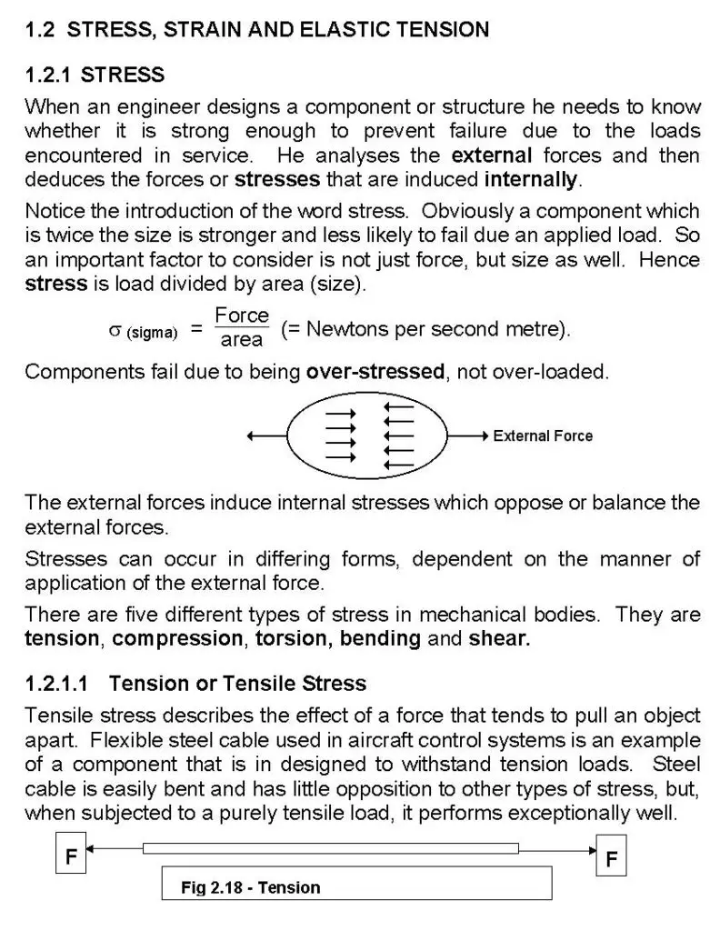
When an engineer designs a component or structure he needs to know whether it is strong enough to prevent failure due to the loads encountered in service. He analyses the external forces and then deduces the forces or stresses that are induced internally.
Notice the introduction of the word stress. Obviously a component which is twice the size is stronger and less likely to fail due an applied load. So an important factor to consider is not just force, but size as well. Hence stress is load divided by area (size).
s (sigma) = (= Newtons per second metre).
Components fail due to being over-stressed, not over-loaded.
The external forces induce internal stresses which oppose or balance the external forces.
Stresses can occur in differing forms, dependent on the manner of application of the external force.
There are five different types of stress in mechanical bodies. They are tension, compression, torsion, bending and shear.
1.2.1.1 Tension or Tensile Stress
Tensile stress describes the effect of a force that tends to pull an object apart. Flexible steel cable used in aircraft control systems is an example of a component that is in designed to withstand tension loads. Steel cable is easily bent and has little opposition to other types of stress, but, when subjected to a purely tensile load, it performs exceptionally well.
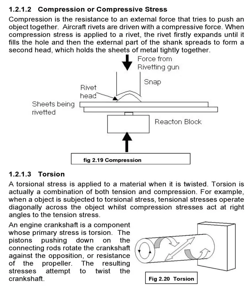
1.2.1.2 Compression or Compressive Stress
Compression
is the resistance to an external force that tries to push an object
together. Aircraft rivets are driven
with a compressive force. When compression stress is applied to a rivet, the
rivet firstly expands until it fills the hole and then the external part of the
shank spreads to form a second head, which holds the sheets of metal tightly
together.
1.2.1.3 Torsion
A torsional stress is applied to a material when it is twisted. Torsion is actually a combination of both tension and compression. For example, when a object is subjected to torsional stress, tensional stresses operate diagonally across the object whilst compression stresses act at right angles to the tension stress.
An engine crankshaft is a component whose primary stress is torsion. The pistons pushing down on the connecting rods rotate the crankshaft against the opposition, or resistance of the propeller. The resulting stresses attempt to twist the crankshaft.
1.2.1.4 Bending Stress
If a beam is anchored at one end and a load applied at the other end, the beam will bend in the direction of the applied load.
An aircraft wing acts as a cantilever beam, with the wing supported at the fuselage attachment point.
When the aircraft is on the ground the force of gravity causes the wing to bend in a similar manner to the beam shown in Fig. 2.21. In this case, the top of the wing is subjected to tension stress whilst the lower skin experiences compression stress. In flight, the force of lift tries to bend an aircraft’s wing upward. When this happens the skin on the top of the wing is subjected to a compressive force, whilst the skin below the wing is pulled by a tension force. The following diagram illustrates this.
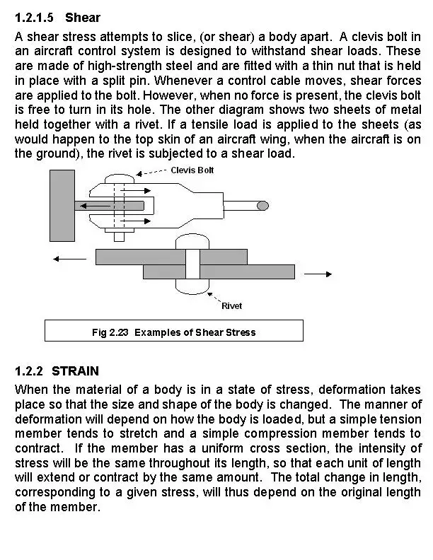
1.2.1.5 Shear
A shear stress attempts to slice, (or shear) a body apart. A clevis bolt in an aircraft control system is designed to withstand shear loads. These are made of high-strength steel and are fitted with a thin nut that is held in place with a split pin. Whenever a control cable moves, shear forces are applied to the bolt. However, when no force is present, the clevis bolt is free to turn in its hole. The other diagram shows two sheets of metal held together with a rivet. If a tensile load is applied to the sheets (as would happen to the top skin of an aircraft wing, when the aircraft is on the ground), the rivet is subjected to a shear load.
1.2.2 Strain
When the material of a body is in a state of stress, deformation takes place so that the size and shape of the body is changed. The manner of deformation will depend on how the body is loaded, but a simple tension member tends to stretch and a simple compression member tends to contract. If the member has a uniform cross section, the intensity of stress will be the same throughout its length, so that each unit of length will extend or contract by the same amount. The total change in length, corresponding to a given stress, will thus depend on the original length of the member.
Deformation due to an internal state of stress is called strain (ε). Any measurement of strain must be related to the original dimension involved.
Example:
Intensity of strain (ε) = change in length (x) / original length (L)
ε = x / L
Where x is the extension or compression of the member.
Note:
Since strain is simply the ratio between two lengths, it is dimensionless. It is, however, usually expressed as a percentage..
Example of Stress and Strain
A steel rod 20 mm diameter and 1m carries a load of 45 kN. This causes an extension of 1.8mm. Calculate the stress and strain in the rod.
Note that there are no units for strain. Strain may also be indicated as a percentage. To show strain as a percentage you simply multiply by 100. So in the above example the strain as a percentage is 0.0018 x 100 = 0.18%.
1.2.3 Elasticity
Engineering materials must, of necessity, possess the property of elasticity. This is the property that allows a piece of the material to regain its original size and shape when the forces producing a state of strain are removed. If a bar of elastic material of uniform cross-section, is loaded progressively in tension, it will be found that, up to a point, the corresponding extensions will be proportional to the applied loads.
This proportionality is known as Hooke’s Law. However, to be meaningful, loads and extensions must be related to a particular bar of known cross-sectional area and length. A more general statement of this law may be made in terms of the stress and strain in the material of the bar.
Within the limit of proportionality, the strain is directly proportional to the stress producing it.
If we plot the graph of stress against strain, we will produce a straight line passing through the origin as shown below. The slope of the graph, stress/strain, is a constant for a given material. This constant is known as Young’s Modulus of Elasticity and is always denoted by the capital letter E. Once the line plotted begins to curve towards horizontal the material is said to have passed its elastic limit and will NOT return to its original length. It will have a permanent stretch.
Young’s Modulus of Elasticity (E) = = the slope of stress/strain graph
The value of E for any given material can only be obtained by carrying out tests on specimens of the material.
For example: For Mild Steel, E = 200 x 109 N/m2 = 200 GN/m2
For Aluminium, E = 70 x 109 N/m2 = 70 GN/m2
Since strain is a ratio and so dimensionless, it follows that E has the same units as stress